Chapter 5: Immunofluorescence and Colour Compensation

5.1 Immunofluorescence

5.1.1 Introduction

Immunofluorescence is the most widespread application of flow cytometry. Given an appropriate antibody, any protein in the cell, which is present in a high enough concentration, can be measured. Several antigens can be measured simultaneously; routinely, most laboratories measure between 3 and 5 antigens although machines have been built which can record up to 17 different colours (Baumgarth and Roederer, 2000). Immunofluorescence can be combined with other stains, for example DNA (See Chapter 6).

5.1.2 Sample preparation

The most important feature of sample preparation, as with all samples for flow cytometry, is the production of a suspension of single cells with few clumps and little debris. Cells from suspension cultures or from peripheral blood present few problems. Cells grown adherent to a culture dish have to be removed from the dish, usually enzymatically. The treatment might alter surface antigens. Lymphoid organs, such as thymus, will usually release single cells after mild mechanical treatment, for example, forcing the tissue through a coarse metal sieve of the type used as a tea strainer. Solid tissues are the most difficult but single cells can usually be obtained by a combination of mechanical stress, incubation with an enzyme or a combination of both.

In clinical samples, if nucleated cells are being studied, the red blood cells are usually lysed either by a brief exposure to distilled water, incubation with an ammonium chloride solution or with a weak detergent.

If surface antigens are to be stained, fresh unfixed cells are reacted with the labelled antibodies. Sometimes the cells are fixed after surface labelling, particularly if an intracellular antigen is also to be stained.

For cytoplasmic or nuclear antigens, the cells must be fixed and permeabilised to give the antibody access to the antigen. There is no standard procedure for staining intra-cellular antigens. Many antigens are adversely affected by some fixatives and consequently the optimum procedure has to be determined for each protein under study. Table 5.1 gives a list of some of the treatments that have been used successfully for different proteins. Several manufacturers sell reagents which are mostly based on permeabilisation in detergent, usually saponin, and fixation in formaldehyde.

Table 5.1. Some methods for permeabilising cells for intracytoplasmic staining

1	Fixation in 70% ethanol at 0°C
2	Fixation in absolute methanol at -80°C
3	Fixation in 1% formaldehyde at 0°C followed by methanol at -20°C.
4	Fixation in 1% formaldehyde in the presence of a detergent at 0°C with or without subsequent fixation in methanol at -20°C.

5.1.3 Staining cells

Cells can be stained either by a direct or an indirect method. In the former, the antibody is labelled with a fluorochrome and incubated with the cells in a single step staining procedure. In the latter, the cells are incubated with the primary antibody, washed and then incubated with a secondary antibody carrying the fluorochrome (Figure 5.1).

Using the direct method, staining cells with several antibodies is straight forward. Washing is not always necessary; the cells can be incubated with the antibodies in a small volume and diluted prior to measurement. When labelling cells in peripheral blood, the diluent often contains a detergent to lyse the erythrocytes. The indirect method can be more sensitive; several secondary antibodies may bind to a single primary molecule. However, multiple antibody staining is more difficult, particularly, as is usually the case, if all the compensation antibodies are mouse monoclonals since the secondary antibody will bind to all the antibodies. A method for staining with a single unlabelled antibody combined with one or more directly labelled antibodies is given in Table 5.2.

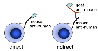
Figure 5.1. Immunofluorescent labelling of cells.

Table 5.2. Combining indirect and direct antibody staining with murine monoclonal antibodies

1) Incubate with unlabelled primary antibody. Wash.

2) Incubate with labelled secondary antibody. Wash.

3) Incubate with mouse serum. (Blocks any unreacted sites on the secondary antibody)

4) Incubate with labelled primary antibodies. Wash.

5) Analyse

When staining for surface and intra-cellular antigens together, it is usual to stain the surface antigens before fixation and permeabilisation. Checks must be made to ensure that the fluorochromes on the surface stains survive any subsequent treatments. Some cell surface antigens will survive the permeabilisation procedure and can be stained simultaneously with the intra-cellular antigens, bearing in mind that the stain will no longer be specific for the surface.

An example is shown in Figure 5.2.

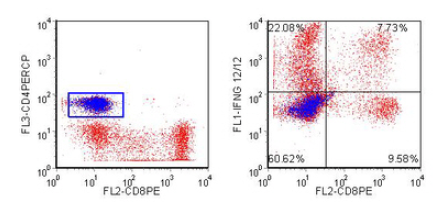
Figure 5.2. Peripheral blood lymphocytes were stimulated using PMA, ionomycin and monensin. They were stained for CD4, CD8, fixed, permeabilised (with Caltag’s Fix and Perm) and then stained for interferon-γ. The CD4 +ve cells are coloured blue. Data supplied by Margaret North and John Farrant, Royal London Hospital. Data file

5.1.4 Selecting the correct concentration of an antibody

Frequently, the manufacturer will recommend the concentration at which to use an antibody. If not, the correct concentration must be determined. This is done by staining positive cells with the antibody at a series of concentrations, usually using 'doubling dilutions', for example, 1:50, 1:100, 1:200, etc. It is helpful to incubate cells with similar concentrations of an isotype control. The type of curve obtained is shown in Figure 5.3. If you want to quantify the number of antigenic sites on the cell, you should use the antibody close to saturation. If the cost of the antibody is an important consideration and you only want to record the number of positive and negative cells, a lower concentration can be selected.

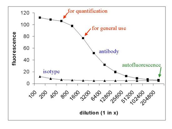
Figure 5.3. A curve that might be obtained when cells are stained with different concentrations of antibody.

5.1.5 Choice of fluorochrome

The fluorochrome selected will depend on what laser is available. Using instruments with an argon-ion laser, fluorescein is usually the first choice, largely because this was the first fluorochrome to be used for immunofluorescence and there is a wide choice of labelled antibodies available. For similar reasons, phycoerythrin (PE) is often chosen as a second colour and one of the tandem conjugates of PE for a third of fourth colour. If other lasers are available, the choice widens considerably (SeeChapter 3).

5.2 Colour compensation

The emission spectra of fluorescent dyes are broad. For example, while fluorescein fluorescence looks, and is, predominately green, the spectrum contains a range of colours from green to red.Figure 5.4 shows the emission spectra of some commonly used dyes. While the peak emission is clearly separated for each dye, there is considerable overlap between the dyes.

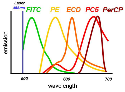
Figure 5.4. Emission spectra for some dyes used to label antibodies. Figure supplied by Graeme Chapman, then at Beckman Coulter, Australia.

Figure 5.5 shows the spectra from fluorescein and phycoerythrin (PE) with two stylised band pass filters superimposed on them. It can be seen that some of the light emitted by fluorescein will be pass through the filter used for PE. This is called spectral overlap.

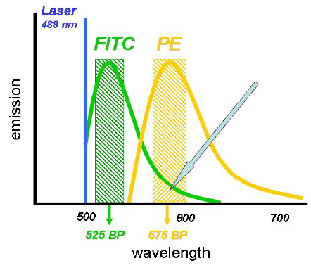
Figure 5.5. Spectra from fluorescein (FITC) and phycoerythrin (PE) with two stylised bandpass filters superimposed. Some of the light from FITC will pass through the filter used to collect light from PE (arrowed).Figure supplied by Graeme Chapman, then at Beckman Coulter, Australia.

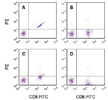
Figure 5.6. Human peripheral blood lymphocytes labelled with CD8-FITC showing the CD4 -ve cells only. A. Uncompensated data. B. Correctly compensated. C. Under compensated. D. Over compensated. Data file

The consequence of this spectral overlap is that cells labelled with FITC will appear to have some phycoerythrin fluorescence. Figure 5.6A shows this effect for human peripheral blood lymphocytes labelled with CD8. The CD8 +ve cells (labelled with FITC) appear to also have PE fluorescence. To obtain a true representation of the data, a correction must be applied. This correction is called colour compensation. We can compensate for the spectral overlap by subtracting a fraction of the fluorescein signal from the PE signal. This has been done to the data shown in Figure 5.6B. In panelC, the data have been under compensated; that is, too little of the fluorescein signal has been subtracted from the PE channel. Panel D shows the effect of over compensation.

Figure 5.7 shows another example. There is spill over of fluorescence from ECD into PE and from PE into ECD. Compensation has to be applied in both directions to represent the data correctly (Note that CD4 and CD8 are mutually exclusive on peripheral blood T cells).

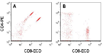
Figure 5.7. Human peripheral blood lymphocytes labelled with CD4-PE and CD8-ECD. A. Uncompensated. B. Compensated data.Data supplied by Graeme Chapman, then at Beckman Coulter, Australia.

There are several ways in which compensation can be set. First the PMT voltages on all the fluorescence channels in use are set to display the data as required; generally to give a good separation between negative and positive cells. Then cells labelled singly with each of the fluorochromes are run and the compensation set by inputting the percentage of the one fluorescence signal that needs to be subtracted from another. Software is available to carry out this procedure automatically, once the data from each fluorochrome has been recorded. For two or three fluorochromes, a manual method is adequate; with four or more colours an automated method should be used.

In machines using analogue electronics, the compensation must be set up correctly before the data is recorded. The necessary subtractions are carried out in the electronics. In more modern machines using digital electronics, the compensation is carried out by software and can be applied off-line after the data has been recorded, an example is shown in Figure 5.8.

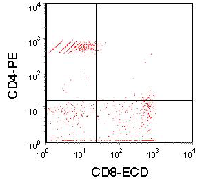
Figure 5.8. Data shown in Figure 5.7 corrected off-line by software. 16% of the ECD signal was subtracted from the PE signal; 30% of the PE signal was subtracted from the ECD signal. The striations in the data are the consequence of subtracting two large digital numbers from each other. In Figure 5.6, the subtraction was carried during data acquisition using analogue values.

If the colour compensation has been applied correctly, the median fluorescence in the PE channel of the fluorescein positive cells will be the same as the median fluorescence of the negative cells. Table 5.3 shows the data from files used in Figure 5.5. The over-and under-compensation are clearly demonstrated. The “correctly” compensated cells are slightly under-compensated, which is what often happens when the compensation is set by eye.

Table 5.3. Median fluorescence in the PE channel, taken from the data in Figure 5.4.

Sample
	FITC -ve	FITC +ve
B	2.86	3.61
C	3.02	7.31
D	2.9	1.33

Note that, in the examples shown, there were negative cells in the sample so that a comparison can be made between the fluorescent and the negative cells. In the absence of these cells, the value for negative cells must be established by running a negative control for each fluorochrome (see Chapter 3, Section 4.4.3). If the compensation is being applied manually, it is best to start with the shortest wavelength and work up to the longest.

The controls for determining the compensation matrix should be as bright as possible and certainly as bright or brighter than the experimental samples. If this is not possible, for example, when investigating a weak antigen, either a different antibody carrying the same fluorochrome or antibody capture beads should be used. The latter are beads carrying anti-mouse Ig antibodies (assuming that a mouse monoclonal is being used); after incubation with the labelled antibody of interest, they will mimic a labelled cell. Once the values for the compensation (sometimes referred to as thecompensation matrix) have been obtained, the PMT voltages must not be altered. If they are, the values in the compensation matrix must be re-determined.

The compensation matrix applies to the particular set of fluorochromes and is applicable to all cells with similar autofluorescence. This statement is not necessarily applicable to tandem dyes (seeChapter 3.2). Energy transfer between the donor and the acceptor molecules is not always complete; there is often some fluorescence from the donor present in the emission spectrum. This is evident inFigure 5.4; both the ECD and PC5 spectrum show some fluorescence from the PE. If antibodies carrying tandem dyes from different manufacturers are used, the compensation matrix should be checked for each antibody.

One consequence of applying compensation is an apparent broadening of the data. This effect can be seen in Figures 5.6 - 9. It results from the subtraction of two comparatively large voltages to give a smaller value (or numbers in the case of digitally compensated data) and the way in which the data is displayed on a logarithmic scale. The data shown in Figure 5.8 was recorded using a Beckman Coulter FC500 with their CXP V.1 program. The data are recorded digitally over a range of 1 to 10 million channels. The negative cells have been recorded at a mean channel number of about 300. As a result of the broadening, in the compensated data, there are cells falling below the negative cells, many of which are apparently negative. The off-axis data can be ‘lost’ from the display by adjusting the scale of the axes, see Figure 5.9C. Although these events cannot been seen on a conventional plot, they will still be recorded when a quadrant region is applied. Various alternative scales have been devised to allow the off-axis events to be visualised (Novo and Wood, 2008). Data displayed using a biexponential scale on the y-axis is shown in Figure 5.9D.

With brightly stained cells, the broadening of the data can give false positives; it has been recommended that curved quadrants are used, which needs suitable software (Roederer, 2001).

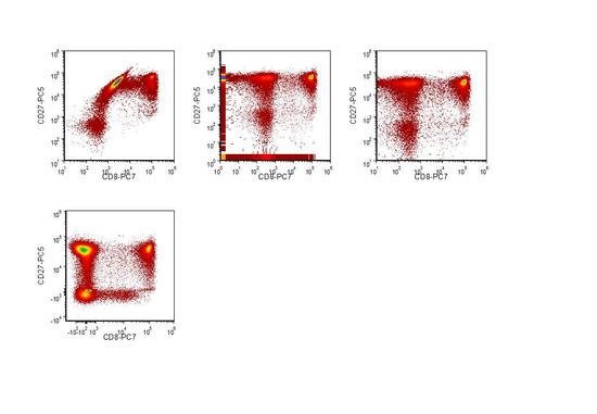
Figure 5.9. Human peripheral blood lymphocytes stained for CD27-PC5 and CD8-PC7. A: Uncompensated data; B: Compensated off-line; C: As B but displayed using a different range on the axes. D: As B but displayed using a biexpontial scale. Data supplied by Martin Adelmann, Beckman Coulter.

Spectral overlap and colour compensation has been discussed above in terms of labelled antibodies. The principles apply equally to any set of fluorochromes, for example when combining immunofluorescence with a stain for DNA (see Chapter 6).

5.3 Antigen quantification

Quantification requires

Use of the antibody at saturation (Figure 5.3, Section 5.1.4) so that all the antigens have an antibody bound to them

Standardised conditions, including environmental factors, such as pH

A method for converting numbers of molecules of fluorochrome into numbers of antibody molecules bound.

There are two methods used. Sets of non-fluorescent beads can be purchased (from Bangs Laboratories, Inc. or BD) that have anti-mouse IgG antibodies on their surface. They have been calibrated so that the number of molecules of mouse IgG that bind at saturation is known. After incubating the beads with the labelled antibody in use, their fluorescence can be measured and the average number of fluorochrome molecules per antibody molecule determined.

If an indirect method is being used, beads coated with calibrated amounts of mouse IgG (from Biocytex, also supplied by Dako) can be used. The beads are incubated with the fluorochrome-labelled anti-mouse IgG. The amount of fluorescence recorded can then be related to the number of mouse antibodies bound to the cell of interest.

The number of molecules of antibody bound to a cell is referred to as the antibody binding capacity (ABC). IgG molecules are bivalent. Depending on steric factors, some of the molecules may bind to two epitopes, others one. Strictly, the ABC can only be related to antigen density if monovalent Fab' fragments of antibody are used. You should also be aware that the binding of an antibody to an antigen can be affected by several factors including steric hindrance and charge. For example, fluorescein carries a negative charge and an antibody labelled with fluorescein may bind only weakly to a negatively charged epitope. Its fluorescence is also sensitive to pH.

A detailed discussion of the problems involved in quantitative fluorescence cytometry can be found in Gratama et al., 1988.

In some circumstances, only the relative numbers of antigens on a cell is required, possibly recorded at different times; an estimation of the absolute numbers of antigens is not necessary. In such cases, the Molecules of Equivalent Soluble Fluorochrome (MESF) can be determined. Fluorescent beads can be purchased that contain a measured numbers of fluorescent molecules, the commonest molecule being fluorescein. The beads are calibrated against of solution of fluorochrome (hence the expression ‘equivalent soluble fluorochrome’). For a given laser power and PMT voltage, the instrument can be calibrated so that channel number in the fluorescence histogram can be converted to fluorescent molecules. The curve shown in Figure 5.10 also serves as a check of amplifier linearity. Once the calibration curve has been established for a particular set of conditions, the sample of interest can be recorded on the same settings and the mean MESF bound to the cells determined.

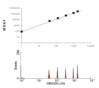
Figure 5.10. A fluorescence histogram and the calibration curve derived from the histogram for beads containing calibrated amounts of fluorescein (shown as MESF in the graph).

From Figure 5.10, you can see that this particular cytometer could detect the equivalent of 100 molecules of fluorescein. This statement does not mean that you could necessarily distinguish between a particle with 100 molecules of fluorescein from one carrying, say, 200 molecules. The separation of two populations depends on the spread of the distribution of fluorescence and the ability to detect a weakly stained population will also depend on the autofluorescence of the cells. All cells fluoresce naturally, due to their components. The autofluorescence from a human lymphocyte excited at 488 nm and recorded at 512 nm is equivalent to about 1000 molecules of fluorescein. Most epithelial cells have far higher autofluorescence, partly due to their larger cytoplasm.

5.4 References

Baumgarth, N. and Roederer, M. (2000). A practical approach to multicolour flow cytometry for immunophenotyping. J. Immunol. Meth 243: 77-97.

Gratama, J.W., D'Hautcourt, J.L., Mandy, F., Rothe, G., Barnett, D., Janossy, G., Papa, S., Schmitz, G. and Lenkei, R. (1998) Flow cytometric quantitation of immunofluorescence intensity: problems and perspectives. Cytometry 33: 166-178.

Roederer, M. (2001) Spectral compensation for flow cytometry: visualization artefacts, limitations, and caveats. Cytometry 45: 194-205.

For further reading on compensation, see Mario Roederer’s Compensation Web Page -www.drmr.com/compensation