Chapter 4: Data Analysis

select the parameters for measurement;
select area, width or height on different parameters (for pulse processing, see Chapter 2.5.2)
adjust the voltages on the PMTs;
adjust the gain settings on the amplifiers;
select logarithmic or linear amplification
select and adjust the threshold (discriminator) settings (see Chapter 2.5.1);
adjust the settings for colour compensation (see Chapter 5.2)
select histograms and cytograms for display;
draw regions and set gates (see below) to be used during data acquisition.

If the flow cytometer can sort cells, the computer controls the sorting process.

As data are acquired, they written to the hard drive to create a file of data, often referred to as ‘listed data’. The computer program can then be used to analyse data subsequent to its acquisition; off-line analysis is useful for the preparation of illustrations for publications, lecture slides, etc.

It is convenient to have a program for analysis of data files on computers in other locations. There are a variety of programs supplied for this purpose; some of them are sold commercially, others are free. Whatever the program used, the principles of data analysis are the same.

4.2 Light scatter

Most instruments measure light scattered by the cells at right angles to the laser beam (side scatter, SS) and light scattered in a forward direction (forward scatter, FS) (see Chapter 2.3.1). The amount of light scattered is affected by the size, shape and optical homogeneity of the cells (or other particles being measured). It is also dependent on the angle at which the scatter is measured. In particular, FS is sensitive to the range of angles over which the light is collected. Consequently the appearance of the FS will depend on the instrument design and may be slightly different in different makes of cytometer.

FS is most sensitive to the size of the cell while SS is most influenced by the optical homogeneity.

4.3 Gating data

To display data from a single parameter, we can use a univariate histogram (Figure 1.1). We can show the correlation between two parameters using a bivariate histogram, or cytogram, in the form of a dot, contour or density plot (Figure 1.2). However, it is impossible to visualise the correlations in multiparameter data, perhaps consisting of as many as 12 fluorescences measured on each cell. We have to adopt a different strategy; we use what are called ‘regions’ and ‘gates’.

Regions are shapes that are drawn around a population of interest on a one- or two-parameter plot. When a region is used to limit the cells that are drawn on a plot, it is termed a gate.

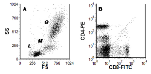
Figure 4.1. Data from human peripheral blood leucocytes. A. Light scatter plot; The clusters labelled G, M & L arise from granulocytes,
monocytes and lymphocytes respectively. B. Plot of two fluorescences. Data file

Figure 4.1 shows two dot plots from some four parameter data derived from human peripheral blood leucocytes. The cells were labelled with anti-CD4-FITC and anti-CD8-PE, both these proteins are expressed on T lymphocytes. The light scatter (SS versus FS) defines three distinct populations; these are the granulocytes, monocytes and lymphocytes, labelled G, M and L. There are at least four sub-populations in the plot of CD4 versus CD8 but we cannot immediately make the link between the different populations shown in the two dot plots.

In Figure 4.2, a region (R1) has been drawn around the lymphocyte cluster in the light scatter cytogram. The computer has coloured the cells in the region red. Any cell falling within this region is also coloured red in all other dot plots created from this data. The colour identifies the lymphocytes in the plot of CD4 versus CD8. This approach is sometimes called ‘colour gating’. Region, R1, can also be used to set a gate on the cytogram of CD4 versus CD8; that is, the computer is instructed to show only the cells that fall in R1; all the cells falling outside R1 are ignored.

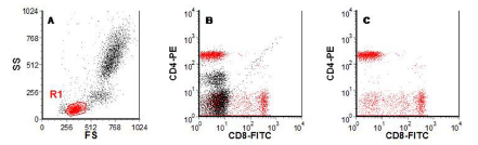
Figure 4.2. As Figure 4.1. A region, R1, has been drawn around the lymphocytes (A). In B, the lymphocytes are coloured red and in C a gate has been set to show only the cells in R1. Data file

A similar procedure can be followed to show the fluorescence of the monocytes (Figure 4.3). A comparison of Figure 4.2 and 4.3 showed that monocytes primarily express CD4 whereas lymphocytes can express CD4 or CD8 but not both on the same cell.

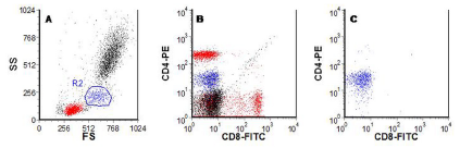
Figure 4.3. As Figure 4.1. A region, R2, has been drawn around the monocytes (A). In B, the monocytes are coloured blue and in C a gate has been set to show only the cells in R2. Data file

Gates can be combined with each other using Boolean logic (AND, OR, NOT). The most common combination is to use gates sequentially. This is equivalent to: IF a cell is in (Gate 1 AND Gate 2) then do something. An example is shown in Figure 4.4, which shows data from human peripheral blood leucocytes stained with anti-CD20-FITC (a B cell marker), CD2-PE (a T cell marker) and CD8-ECD (a marker for cytotoxic T cells). A region (Lymphs) was drawn around the lymphocytes on the scatter plot (A). This region was used to set a gate on a plot of CD2 versus CD20 fluorescence (B). A further region (T cells) was set on the CD2+ve, CD20-ve cells. Both regions were used to gate a display of CD2 versus CD8 fluorescence (C). The cells displayed were in region (Lymphs) AND region (T cells); all other cells were excluded. The CD8 +ve, CD2 +ve cells are arrowed.

Figure 4.4. Human peripheral blood leucocytes stained with CD20-FITC, CD2-PE and CD8-ECD. For further information, see the main text. Data file

Figure 4.5 shows an example using a NOT gate, which allowed the separation of cells from G1 and G2/M of the cell cycle to be separated from the S phase cells. For further discussion, see Chapter 8.

Figure 4.5. Chinese Hamster V79 cells incubated for 30 min with BrdUrd. The cells were fixed and stained with an antibody to BrdUrd
and propidium iodide (PI). A region, labelled ‘S phase, was pl aced on the BrdUrd +ve cells (A). Panel B shows the DNA histogram. Panel C shows the cells which were NOT in S phase giving the G1 and G2 cells. Data supplied by G. D. Wilson, Detroit. Data file

4.3.1 Back gating

It is normal practice to set a gate on displays of fluorescent parameters using a region around a selected population defined on a light scatter cytogram. However, occasionally, it is unclear as to where the region should be drawn. In such cases, a region can often be drawn on a fluorescence parameter, which defines the population of interest, and the region used to set a gate on the light scatter plot. The scatter can now be seen more clearly so that the correct region can be set, in turn, to use as a gate in the normal manner.

The process is illustrated in Figure 4.6. Figure 4.6a shows the ungated data from some human ovarian carcinoma cells spiked with peripheral blood. They have been labelled with an antibody to the ovarian cells, Ber-EP4-FITC. It is not clear where to draw a region on the scatter plot to define the carcinoma cells. In Figure 4.6b, a region has been drawn around the Ber-EP4 positive cells and this has been used to gate on the light scatter plot (Panel C). This plot can be used to set a region for the light scatter gate for the epithelial cells. It will include some granulocytes but will have excluded the bulk of the leukocytes.

Figure 4.6a. Human carcinoma cells plus peripheral blood. A. Scatter plot (note that the side scatter is logarithmic). B. Side scatter versus Ber-EP4-FITC. (Some of the larger epithelial cells are off-scale on the FS axis. With hindsight, the FS should have been measured on a log scale). Data supplied by Martin Forster, Institute of Cancer Research, UK. Data file

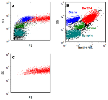
Figure 4.6b. For details, see Figure 4.6a. In Panel B, a region has been drawn around the Ber-EP4 positive cells. This region has then been used to gate on the light scatter plot (C). The leucocyte subsets have also been identified on the basis of their side scatter and lack of expression of Ber-EP4. Data file

4.4 Statistical analysis

4.4.1 Intensity and spread of a distribution

Two measures are generally made of a distribution, intensity and spread. In flow cytometry, the intensity of a distribution can be represented by the position of the “centre” of the distribution. The “centre” is usually represented mathematically by the mean, median or peak channel number.

If the data has been displayed on a linear scale, the arithmetic mean is used; for logarithmically displayed data, the geometric mean is generally chosen. If any part of the distribution lies off scale at either end of the axis, the value for the mean channel number will be inaccurate and should not be used; the median channel can be used as long as more than half of the distribution in on scale. The peak channel number is an inaccurate measure of the centre of a distribution and is not recommended. For a Guassian (normal) distribution, these three values should be equal.

The spread of a distribution is usually expressed as the Standard Deviation (SD). However, in flow cytometry, the coefficient of variation (CV) is preferred because it is dimensionless and, on a linear scale, does not depend on where in the histogram the data is recorded.(CV = SD/mean channel number).

4.4.2 Numbers of cells in a sub-population

Frequently the percentage of cells in a sub-population is required. In immunofluorescence analysis, quadrants are often drawn on a cytogram and the number of cells in each quadrant recorded. InFigure 4.7, a quadrant has been set to delineate the CD4 +ve, CD8 +ve and the negative population. While quadrants are often convenient to use, they are not always required Figure 4.8shows an example where polygonal regions are more appropriate.

Figure 4.7. Quadrant regions showing the percentage of cells in each sub-population.

Figure 4.8. Neuroblastoma cells incubated with BrdUrd and labelled with an anti-BrdUrd antibody and propidium iodide, which binds to DNA and shows the cell cycle. Polygonal regions have been used to define the +ve and -ve cells. For further information about this method, see Chapter 8.

While flow cytometry generally gives the percentage of a particular sub-set of cells, some flow cytometers precisely record the the volume of sample analysed or deliver a fixed volume of sample. A percentage count of a sub-population of cells can be directly converted to an absolute count. In instruments without this facility, two approaches are used to measure the absolute count, referred to as two platform or one platform methods.

In the two platform approach, the concentration of all the cells in a sample is determined by another method. For blood leucocytes, a haematology counter is used. For cultured cells, an electronic sizing (Coulter) counter may be used. The flow cytometer is then used to determine the percentage of cells in a particular sub-set so that the cell concentration of the sub-set can be calculated. The disadvantage of the two platform method is that errors in the two instruments are compounded and that two instruments are required. In the one platform method, an absolute cell count is performed on the cytometer. Some instruments allow a fixed volume of sample to be analysed, which will give an absolute count directly. In most cytometers, a fixed volume of sample is spiked with a known number of fluorescent beads. (Suitable beads with an assayed concentration may be obtained from Beckman Coulter; alternatively, tubes containing known numbers of lyophilised beads are sold by BD). The brightness and light scatter of the beads is different to that of cells so that beads and cells can be easily distinguished in the flow cytometer. Counting the number of beads in the portion of the sample analysed allows the volume analysed to be calculated and hence the concentration of cells. The disadvantage of this method is that beads can stick to each other and to the walls of the tube leading to an underestimation of the bead count.

4.4.3 Determination of positive

When recording the percentage of positive cells, we need to distinguish between negative and positive staining, that is, to define the negative population. To define the negative cells, unstained cells are inadequate; they will only correct for autofluorescence and ignore any fluorescence resulting from non-specific binding to the cells.

If the sample contains negative cells as, for example, in Figure 4.4, the control is built into the sample and a further control is often unnecessary. If the samples does not contain negative cells, people have traditionally used an isotype control. For example, if cells are stained with a fluorescein-labelled mouse IGg1 antibody, labelled IgG1 fraction is used as the control. This control can be erroneous unless the fluorescence to protein ratio is the same for the specific antibody and the non-specific control. For multi-colour experiments, the use of ‘fluorescence minus one’ (FMO) is recommended (Roederer, 2000). An example of the controls used in a simple four colour stain is shown in Table 4.1.

Table 4.1. Samples needed for the negative controls in a four colour experiment.

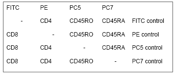
Figure 4.9 shows a stain for CD4. There are other, negative lymphocytes present; the distinction between positive and negative is clear; a further negative control is superfluous.

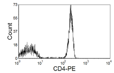
Figure 4.9. CD4 on lymphocytes; clear separation between positive and negative cells.

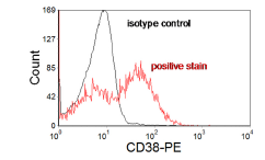
Figure 4.10A. CD38 in leukaemia. The distinction between positive and negative is unclear. Data file

In Figure 4.10A, the positive and negative populations overlap and a negative control is needed to estimate the fraction positive. In this sample, an isotype control was used. Sometimes, it is helpful if the isotype control is subtracted from the positive sample using, for example, the method first described by Overton (1985), see Figure 10B.

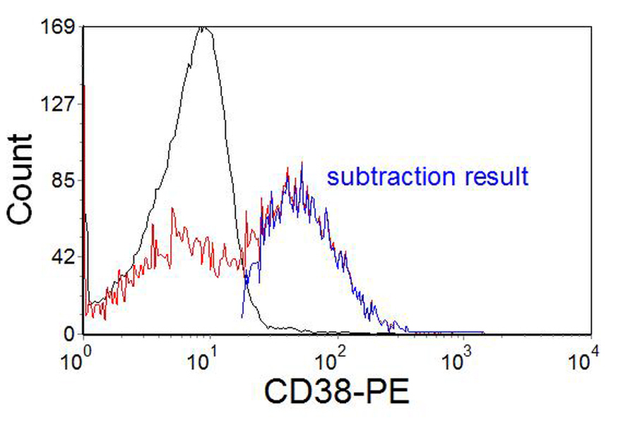
Figure 4.10B. CD38 in leukaemia. The same data as in Figure 10 A, showing the result of histogram subtraction.

In the data shown in Figure 4.11, there is only a single population present. It is sometimes the practice to put a marker on the negative control to include, say, 98% of the cells and to record any staining greater than this in the positive sample as being positive, which would be valid for the data in Figure 4.10. In this case, it is clearly not valid. All the cells are positive; it is the degree of positivity which should be recorded, preferably the Molecules of Equivalent Soluble Fluorochrome (MESF) (see Chapter 5, Section 3).

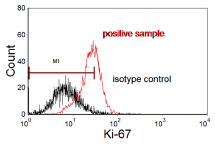
Figure 4.11. Ki-67 expression in breast carcinoma cells from a fine needle aspirate. The marker, M1, covers 98% of the negative cells. The positive cells overlap with the isotype control. Data file

4.5 Detection of rare events

Flow cytometry is well suited to the detection of rare events. If suitable markers are available to separate the cells being analysed from the other events, as few as 1 cell in 10⁷ can be measured. In order to achieve a count of the desired statistical significance, only the total number of positive events (n) is relevant. In the absence of any background, the standard deviation (SD) will be equal to √n. For a CV of 3%, 1000 positive cells need to be counted. If there are non-specific events present, this number increases. If ‘a’ events are recorded from the positive sample and ‘b’ from the negative control, the SD is √(a + b). Increasing the number of identifying markers will, generally, improve the separation of the positive cells from the bulk population and increase the precision of the measurement.

Applications, in which the principles of rare event analysis are applied, can be found in Chapter 7,Sections 7.3, 7.4, 7.8 and 7.12.

Another application is in the detection of tumour cells in the bone marrow and peripheral blood of patients with cancer.

4.6 References

Overton, W.R. (1988) Modified histogram subtraction technique for analysis of flow cytometry data. Cytometry, 9:619-26. Erratum in Cytometry, 10:492-4, 1989.

Roederer, M., (2001) Spectral compensation for flow cytometry: visualization artifacts, limitations, and caveats. Cytometry, 45:194-205.